This section looks at alpha, beta and gamma decay. First ensure you are happy with the basic idea of radioactive decay rates reviewed in Section 1 and the Q-factor discussed in Section 2.

Alpha Decay

Some heavy nuclei are found to be unstable to the ejection of a helium 4-nucleus (2 protons and 2 neutrons), known as alpha decay ($\alpha$-decay). This tends to occur for heavier nuclei, particularly those where the proton-to-neutron ratio is too high (recalling that larger nuclei require an excess of neutrons to overcome the Coulomb force.) The process is spontaneous, i.e. it doesn’t need to be triggered by anything. Below we will study some basic properties of $\alpha$-decay, before looking at the underlying quantum physics.

Energetics

Alpha decay can only occur if the energetics are favourable. We require that the binding energies of the resultant daughter particles sum to more than the binding energies of the parent particle. The generic equation for $\alpha$-decay is:

$${}_Z^A{\text{X}}_N\to {}_{Z-2}^{A-4}{\text{Y}}_{N-2}+\alpha ,$$

where we can see that the parent nucleus has lost 4 units of atomic mass number (A) and 2 units of atomic number (Z), and where

$$\alpha ={}_2^4{\text{He}}_2.$$

By conservation of mass-energy: $$m_X{c}^2=m_Y{c}^2+T_Y+m_{\alpha }{c}^2+T_{\alpha },$$

where $T_Y$ is the resulting kinetic energy of the daughter nucleus and $T_{\alpha }$ is the kinetic energy of the $\alpha$ particle. We define the Q-factor as the sum of the kinetic energy released $$Q=T_Y+T_{\alpha },$$

such that $$Q=(m_X-m_Y-m_{\alpha })c^2.$$

The total numbers of protons and neutrons does not change, so the Q-factor really depends on the differences in binding energies between the parent and daughter particles, $$Q=(B_{\alpha }+B_Y-B_X).$$

Since we cannot have negative kinetic energy, it must be the case that $Q>0$ and $\alpha$-decay cannot otherwise occur. So we require that the combined binding energy of the daughter particles is greater than the parent particle, i.e. they are more tightly bound. Recalling that binding energy is really a negative thing, this releases kinetic energy which goes into the daughter particles. This is also explains why emission of other sized groups of protons and neutrons mostly does not occur (with one or two rare exception), these are less tightly bound and hence the calculations for these hypothetical decays would give $Q<0$.

For example, $${}_{90}^{228}\text{Th}\to {}_{88}^{224}\text{Ra}+\alpha$$

has a Q-value of $5.5\mathrm{M}\mathrm{e}\mathrm{V}$, whereas a decay resulting in the emission of a proton, rather than an $\alpha$ particle,

$${}_{90}^{228}\text{Th}\to {}_{87}^{227}\text{Ac}+{}_1^1\text{H}$$

has a Q Value of $-6.4\mathrm{M}\mathrm{e}\mathrm{V}$, i.e. it cannot occur.

Therefore, we can see that it is the very high binding energy (i.e low mass) of an $\alpha$ particle ($28.3\mathrm{M}\mathrm{e}\mathrm{V}$) that is the reason for this particle to be ejected, since this makes $Q>0$ more likely.

Nuclides which decay by $\alpha$-decay are those with a deficit of neutrons (excess of protons) with respect to the line of stability. (Recall that larger nuclei require $N\approx 1.4Z$ to be stable due to the effect of the Coulomb interaction). $\alpha$-decay moves the daughter particle slightly closer to the line of stability as the required excess of neutrons is smaller for lighter nuclei. We usually find that $Q>0$ only occurs for $A>150$, and $Q\approx 6\mathrm{MeV}$ is typical.

Features of Alpha Decay

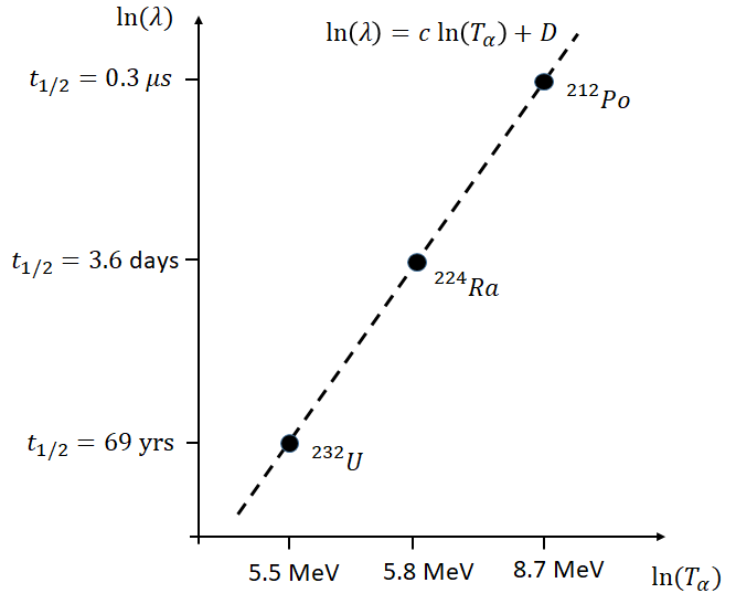
We find that there is a structure to the observed kinetic energy of the $\alpha$ particles: the energies are found to take one of a set of discrete energies rather than continuous spectrum. We also observe an enormous range in the decay rates of different nuclei by $\alpha$-decay. This range is from ${10}^{-7}\mathrm{s}$ to ${10}^{10}\mathrm{y}\mathrm{e}\mathrm{a}\mathrm{r}\mathrm{s}$, some 24 order of magnitude. Any model we develop should therefore explain these two experimental observations.

Geiger and Nuttall found, in 1911, a simple empirical relationship between the decay constant, $\lambda$, and the $\alpha$ particle kinetic energy, $T_{\alpha }$, $$\ln (\lambda )=c\ln (T_{\alpha })+D$$

where $c$ and $D$ are fitted constants. Remarkably, this relationship holds roughly true over a huge range of decay constants and energies. This is illustrated in Figure 2, where it should be remembered that $t_{1/2}=\ln (2)/\lambda$.

Alpha Decay Energetics

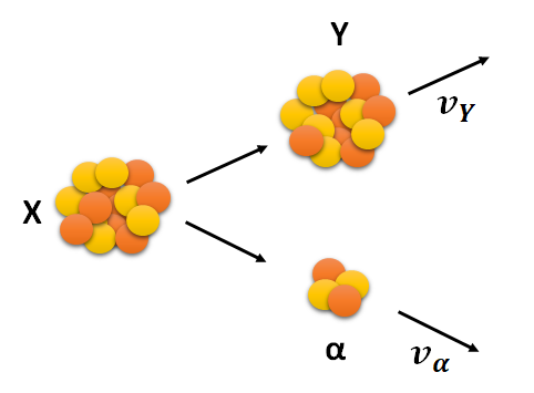
Since the $\alpha$ particle is much lighter than the daughter nucleus, most of the energy released by $\alpha$ decay goes into kinetic energy of the $\alpha$ particle (i.e. $T_{\alpha }\gg T_Y$). We can perform this calculation for a specific decay as follows.

Consider the decay: $${}_{84}^{214}\text{Po}\to {}_{82}^{210}\text{Pb}+\alpha$$

The binding energies of ${}_{84}^{214}\text{Po}$, ${}_{82}^{210}\text{Pb}$ and $\alpha$ are 1.66601 GeV, 1.64555 GeV, and 28.296 MeV, respectively. The Q-value for this decay is therefore: $$Q=B_{Pb}+B_{\alpha }-B_{Po}=1.64555\mathrm{GeV}+28.296\mathrm{MeV}-1.66601\mathrm{GeV}=7.82\mathrm{MeV}$$

This is positive, as it must be for $\alpha$-decay to occur.

If all this energy went to the $\alpha$ particle it would have a speed of $$v=\sqrt{\frac{2Q}{m}}=\sqrt{\frac{2\times (7.82\mathrm{MeV})}{3727.37\mathrm{MeV}/{\mathrm{c}}^2}}=0.0042c\approx 1260\mathrm{km}/\mathrm{s},$$

where we used that $m_{\alpha }=3727.37\mathrm{MeV}/{\mathrm{c}}^2$. The speed, while large, is much less than $c$, and so no relativistic corrections are required here.

In reality, some of the energy will go into kinetic energy of the daughter nucleus. We can see how much using conservation of momentum. Working in the rest frame of the parent nucleus, we have: $$m_Y{v}_Y=-m_{\alpha }{v}_{\alpha },$$ where we have denoted the daughter nucleus with $Y$. Hence the ratio of the speeds is $$\frac{v_{\alpha }}{v_Y}=\frac{m_Y}{m_{\alpha }}.$$ In the case of the reaction above this ratio is approximately the ratio of atomic mass numbers, $210/4\approx 52$. In terms of energy: $$\frac{E_{\alpha }}{E_Y}=\frac{m_{\alpha }{v}_{\alpha }^2}{m_Y{v}_Y^2}=\frac{m_{\alpha }}{m_Y}\frac{m_Y^2}{m_{\alpha }^2}=\frac{m_Y}{m_{\alpha }}.$$

and so the same ratio applies, 98% of the energy goes to the $\alpha$ particle.

The Coulomb Barrier

To understand the decay rates of different nuclei by $\alpha$-decay, we must understand what prevents nuclei simply decaying in the cases where $Q>0$. In order for a single nucleus to split into a daughter nucleus and an alpha particle, we can imagine an intermediate state where the $\alpha$ particle and the daughter nucleus have just split apart, but are still close enough for the strong interaction to be a consideration. We can therefore think of the formed $\alpha$ particle sitting in the potential well of the nucleus, as shown in Fig 3. Note that here the potential well is due to both the strong nuclear interaction and the Coulomb interaction.

In order to be free of the nucleus, the $\alpha$ particle must pass through a potential barrier. Classically it does not have sufficient energy, and this is only possible using quantum mechanical tunnelling, i.e. due to the wavefunction being non-zero beyond the barrier. (If the energy was above the barrier than the decay would have happened almost immediately and we wouldn’t observe it). This explains the random nature of the decay. It also explains the huge range in decay rates.

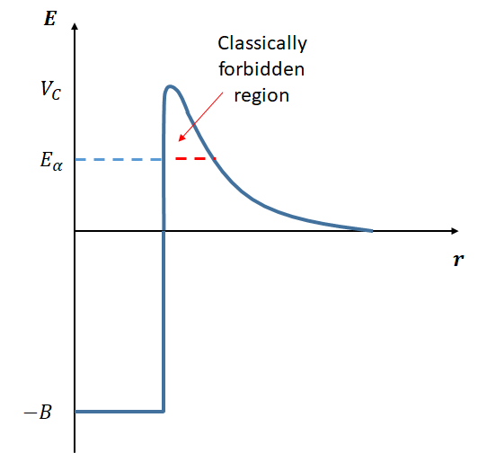
This potential barrier is sometimes called the Coulomb barrier, although this can be slightly confusing because the Coulomb force is tending to push the $\alpha$ particle away from the nucleus, it is really the strong interaction that needs to be overcome.

Working semi-classically, we can imagine the $\alpha$ particle ‘bouncing’ within the well, reflecting off the barrier with frequency $f$. If the probability of tunnelling through the barrier at each strike is $P$ then the decay rate $\lambda$ can be approximated simple as

$$\lambda =fP.$$

We can estimate $f$ to be roughly $v/a$, where $v$ is the speed of the $\alpha$ particle as it bounces between the walls (related simply to its kinetic energy, $K$, and mass $m$ by $v=\sqrt{2mK}$.

We can obtain a rough estimate the height of the barrier by computing the Coulomb potential between an alpha particle and the daughter nucleus that are just touching,

$$U=k\frac{q_1{q}_1}{r}=k\frac{2(Z-2)e^2}{r}$$ We obtain an estimate of their radii using $r=r_o{A}^{1/13}$ and hence the separation of their centres when just touching is the sum of the two radii.

For example, for the decay

$${}_{83}^{211}\text{Bi}\to {}_{81}^{207}\text{X}+\alpha$$ the daughter nucleus has $A=207$ and the $\alpha$ particle, as always, has $A=4$. The two radii can be estimated using $$r_X=(1.2\mathrm{fm})A^{1/3}=7.1\mathrm{fm},$$ and $$r_{\alpha }=1.9\mathrm{fm},$$ giving a separation of $9.0\mathrm{fm}$.

We then estimate the Coulomb barrier height as $$U=k\frac{2(Z-2)e^2}{r}=(9\times {10}^9)\frac{2(81-2)(1.6\times {10}^{-19}{)}^2}{9\times {10}^{-15}}=4.0\times {10}^{-12}\mathrm{J}=25\mathrm{MeV}.$$

As expected, this is (several times) larger than the typical kinetic energies of $\alpha$ particles (and so several times larger than the Q-value). Therefore, classically, this barrier cannot be penetrated (otherwise the decay would be immediate), and so $\alpha$-decay requires quantum tunnelling. This is what leads to the stochastic (random) nature of $\alpha$-decay.

To determine the probability of the $\alpha$ particle tunnelling through the Coulomb barrier we need to solve the Schrodinger equation and hence integrate the square of the wavefunction beyond the barrier. This is quite difficult, and you are not expected to do this, but some of the details can be found in Krane Section 8.4. For interest, the result is that the probability is given by

$$P=\exp (-2G)$$

where $G$, the Gammow factor, is given by $$G=\sqrt{\frac{2m}{{\hslash }^2}}{\int }_a^b[V(r)-Q{]}^{1/2}dr$$

where $a$ is the radius of the well, $b$ is the distance at which the $\alpha$ particle would be classically free (i.e. its kinetic energy is above the potential), $Q$ is the kinetic energy of the $\alpha$ particle, $m$ is its mass, and $V(r)$ is the height of the Coulomb barrier.

The important thing to note here is that the probably depends on the exponential of the Gammow Factor, which itself depends on the $\alpha$ particle energy. This shouldn’t be surprising, the exponential came up when you studied the finite square well.

Due to the exponential, small changes in the Q-value therefore lead to a huge change in the probability and hence a huge change in the decay rate and half life. In fact a change in the Q-value by a factor of 2 can change the half life from a tiny fraction of a second to the age of the Universe.

Beta Decay

Beta Decay ($\beta$-decay) is the emission of an electron or a positron from the nucleus. If the nucleus has an excess of neutrons, a neutron can decay into a proton and an electron - the protons remains in the nucleus and the electron is emitted. This is referred to as Beta-minus, ${\beta }^{-}$, decay. Similarly, a proton can decay in a neutron and a positron, with the positron emitted, known as Beta-plus (${\beta }^{+}$) decay. Both of these decays are mediated by the weak interaction, which you will study later in the module.

A positron is the anti-particle of an electron, it has identical mass but opposite charge. The positron will quickly annihilate with any electron encountered. This results in the emission of two gamma rays, each of energy 0.511 MeV (the rest energy of the electron/positron) emitted in (almost) opposite directions. This is convenient for the technology called Positron Emission Tomography (PET) as detecting these two photons allows the emission to be localised and hence a 3D image (tomogram) to be created. Those of you taking Medical Physics will learn more about this.

Unlike in alpha decay, where discrete values of energy are released, the emitted electron or positron has a range of possible energies up to some maximum. The maximum is the Q-value of the decay, i.e.

$$Q=m_X-m_Y-m_e$$ where $m_X$ and $m_Y$ are the masses of the parent and daughter nuclei, respectively. As for $\alpha$-decay, the Q-value must be positive, meaning that the daughter nucleus must be more tightly bound (more stable) than the parent.

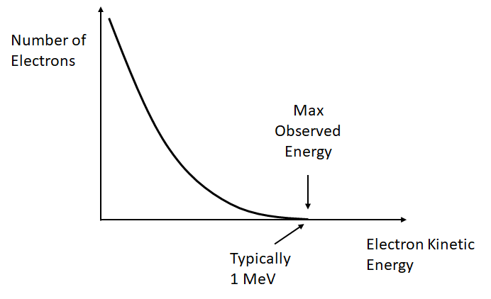
At first sight it is quite strange that the electron/positron does not take practically all of the energy (with a small amount going to the much more massive nucleus) - where does it go? This was a mystery for some time, and led to the discovery of neutrinos.

Neutrinos

Beta decay is always accompanied by the emission of an electron neutrino. ${\beta }^{-}$ decay results in the emission of an anti-neutrino, ${\beta }^{+}$ decay results in the emission of a neutrino. You will study neutrinos in the particle physics section of the module, but here you should be aware that they are uncharged and have a very small rest mass ($<1\mathrm{e}\mathrm{V}$) We know they must be emitted because:

1. The neutrino carries away some energy, allowing for the observed spectrum of energy for the electrons/positrons

2. Without the neutrino, we do not conserve spin

For ${\beta }^{-}$ decay, the process is $$n\to p+e^{-}+\overline{{\nu }_e},$$

while for ${\beta }^{+}$ decay, the process is $$p\to n+e^{+}+{\nu }_e,$$

where ${\nu }_e$ and $\overline{{\nu }_e}$ are the (electron) neutrino and anti-neutrino, respectively. There is a third possible decay called electron capture, $$p+e^{-}\to n+{\nu }_e,$$ where one of the orbital electrons is absorbed into the nucleus. This has the same net effect as ${\beta }^{+}$ decay as the positron from the ${\beta }^{+}$ decay will annihilate with an electron. Positron capture, while technically possible, is hindered by the lack of positrons in normal environments.

Examples of Decays

In ${\beta }^{+}$ decay a nucleus converts a proton intro a neutron, while in ${\beta }^{-}$ decay a nucleus converts a neutron into a proton. ${\beta }^{+}$ decay therefore occurs for nuclei with an excess of protons and ${\beta }^{-}$ decay for nuclei with a deficit of protons with respect to the line of stability. There is no change in the nucleon number, $A$.

For example, Cobalt-60 decays into Nickel-60 by ${\beta }^{-}$ decay with a half-life of 5.27 days, reducing its excess of neutrons: $${}_{27}^{60}\text{Co}\to {}_{28}^{60}\text{Ni}+e^{-}+\overline{{\nu }_e}.$$

An example of ${\beta }^{+}$ decay is: $${}_{91}^{230}\text{Pa}\to {}_{90}^{230}\text{Th}+e^{+}+{\nu }_e.$$

Equivalently, we could have electron capture: $${}_{91}^{230}\text{Pa}+e^{-}\to {}_{90}^{230}\text{Th}+{\nu }_e.$$

Beta Decay Chains

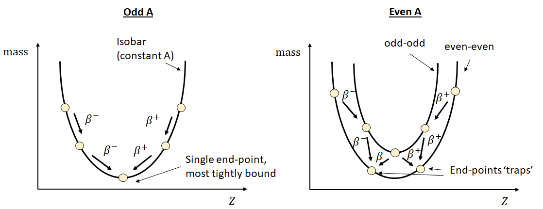
For a nucleus that is some way from the line of stability, multiple $\beta$ decays may occur. These take a slightly different form if the original nucleus has odd or even $A$. (Recalling that $\beta$-decay does not change $A$, so the daughter particles will have the same $A$). The difference can be explained by reference to the SEMF formula. For a nucleus with odd $A$, each decay toggles the nucleus between being and even-even and an odd-odd nucleus. This leads to a significant change in binding energy and a ‘zig-zag’ pattern, as shown in Figure 5. For even $A$ nucleus, there are two different end-points, depending on which decay path was followed. Even though one of these end-points is lower, $\beta$ decay between them is not possible - $\beta$-decay takes us from an even-even to an odd-even, not a different even-even, and going via an odd-even would decrease the binding energy, i.e. going ‘uphill’.

Gamma Decay

We will not study Gamma Decay ($\gamma$-decay) in detail in this module, but you should know the following:

• $\gamma$-decay is the emission of a photon from the nucleus due to a change in its internal energy state.

• $\gamma$-ray energies range from a few keV to 8 MeV.

• $\gamma$-decay is usually the by-product of another decay which leaves the daughter nucleus in an excited state. When the nucleus relaxes to the ground states, a photon is emitted.

• While $\gamma$ decay usually occurs almost instantly (${10}^{-12}\mathrm{s}$), some excited states are metastable, meaning that the $\gamma$ emission is delayed by some period of time. The most famous is Technicium-99m, ${}^{99m}\mathrm{T}\mathrm{c}$, where the ‘m’ stands for a metastable state created when Mo-99 decays via $\beta$ decay. Technicium-99m has a half life of about 6 hours and emits photons with an energy of 140 keV, two properties which turn out to be ideal for use as a tracer for medical imaging. Those taking medical physics will discover much more about this when studying nuclear medicine and gamma cameras.